Logistic Regression applies to almost all classification tasks in real world, as it can consume either discrete and continuous features, it can handle millions and billions of features, it can be trained real quick and it has strong interpretations.
1. Introduction
Logistic regression is one of the most widely used machine learning algorithms in industries, given its simplicity and interpretable form.
2. Mathematical Basis
We know that supervised learning could be regarded as the process of learning some kinds of mapping \(f\) between input \(X\) and output \(y\): \(y = f(X)\). And logistic regression is a simple linear model for classification problems, which means \(f\) is linear.
2.1 Probabilistic Motivation
We start from simplest case where there are only two classes, the output \(y\) is binary: \(y\in \{0, 1\}\), if we consider it as a random variable, we will have \(Y\sim \text{Bernoulli}(p)\) with probability mass function
\[
f(y) = p^{y}(1-p)^{1-y},~\text{where }y\in\{0,1\},~p\in[0,1],
\]
then from the probabilistic perspective, we would like to modeling the probability of the output to be positive (actually this is the parameter of the Bernoulli distribution above), i.e.
\[
P(y=1|x)=p(x)=\hat{y}.
\]
We could build a linear regression model between \(x\) and \(p(x)\). However it could happens that for some ranges of \(x\), \(p(x)\) is out of \([0,1]\), that’s hard to interpret. More over, the most important thing is the distribution of target is binomial rather than normal distribution. One of the ideas is use a function to map \(p(x)\) within \([0,1]\). And one of the choice of the function is called sigmoid function \(\sigma(x)\),
\[
\sigma(x) = \frac{1}{1+e^{-x}},
\]
with derivative
\[
\sigma’(x) = \frac{e^{-x}}{(1+e^{-x})^{2}} = \frac{1}{(1+e^{-x})} \frac{e^{-x}}{(1+e^{-x})} = \sigma(x)\left( 1 - \sigma(x)\right)
\]
It’s a “S”-shaped curve where \(\sigma(x)\) is close to 0 for \(x\) goes to \(-\infty\) and close to 1 for \(x\) goes to \(+\infty\).
Therefore logistic regression is actually modeling the probability of outputs to be one of the classes (discriminative model),
\[
\begin{aligned}
P(y = 1|\mathbf{x}) &= \sigma(\mathbf{x}^{\top}\mathbf{w}), \\
P(y = 0|\mathbf{x}) &= 1 - \sigma(\mathbf{x}^{\top}\mathbf{w}) = \sigma(-\mathbf{x}^{\top}\mathbf{w}),
\end{aligned}
\]
here \(x\) is a row vector of predictors, \(\mathbf{w}\) is a column vector consists of coefficients of logistic regression. Now assume we have a \(n\times p\) input matrix \(\mathbf{X}\), represents for \(n\) observations and \(p\) features (predictors), where \(\mathbf{x}_{i}\) is the \(i\) th row; an output vector \(\mathbf{y}\) with length \(n\). For observation \(i\) (vector \(\mathbf{x}_{i}\)), we have
\[
P(y_{i} = 1|\mathbf{x}_{i}) = \frac{1}{1+e^{-\mathbf{x}^{\top}_{i}\mathbf{w}}},
\]
then with logarithm transformation,
\[
\begin{aligned}
&\frac{P(y_{i} = 1|\mathbf{x}_{i})}{P(y_{i} = 0|\mathbf{x}_{i})} = \frac{1}{e^{-\mathbf{x}_{i}^{\top}\mathbf{w}}} = e^{\mathbf{x}_{i}^{\top}\mathbf{w}} \\
\Longrightarrow &\log\left(\frac{P(y_{i} = 1|\mathbf{x}_{i})}{P(y_{i} = 0|\mathbf{x}_{i})}\right) = \log\left(\frac{\hat{y_{i}}}{1-\hat{y_{i}}}\right) = \mathbf{x}_{i}^{\top}\mathbf{w}.
\end{aligned}
\]
This form is similar to linear regression \(\mathbf{y} = \mathbf{X}\mathbf{w} + \epsilon\), the difference is the target is the log odds ratio rather that raw target. As we can notice, log odds ratio (a.k.a logit function) is the inverse of sigmoid function**.
2.2 Parameters Estimation
Next we will try to estimate the coefficients \(\mathbf{w}\). In linear regression with probabilistic view, we use the idea of Maximum Likelihood Estimate (MLE) which means parameters (coefficients) should make the likelihood of the observed data to be maximum, i.e.,
\[
\hat{\mathbf{w}} = \arg\max_{\mathbf{w}} f(\mathbf{X}, \mathbf{y}|\mathbf{w})
\]
here we can take condition on \(\mathbf{X}\) since that’s the information we know, therefore we get,
\[
\hat{\mathbf{w}} = \arg\max_{\mathbf{w}} f(\mathbf{X}, \mathbf{y}|\mathbf{w}) = \arg\max_{\mathbf{w}} f(\mathbf{y}|\mathbf{X}, \mathbf{w})f_{X}(\mathbf{X}) = \arg\max_{\mathbf{w}} f(\mathbf{y}|\mathbf{X}, \mathbf{w}).
\]
Hence, for logistic regression, the coefficient should be
\[
\hat{\mathbf{w}} = \arg\max_{\mathbf{w}}f(\mathbf{y}) = \arg\max_{\mathbf{w}}\prod^{n}_{i=1}f(y_{i})
\]
since we assume the observations are independent.
The likelihood function we are look for is
\[
L(\mathbf{w}) = \prod^{n}_{i=1}f(y_{i}) = \prod^{n}_{i=1}\left(1-\hat{y_{i}}\right)^{1-y_{i}}\hat{y_{i}}^{y_{i}},
\]
take the logarithm, we have
\[
\begin{aligned}
\log L(\mathbf{w}) =~&\sum^{n}_{i=1}(1-y_{i})\log\left(1-\hat{y_{i}}\right) + \sum^{n}_{i=1}y_{i}\log p(\mathbf{x_{i}}) \\
=~&\sum^{n}_{i=1}\log\left(1-\hat{y_{i}}\right) + \sum^{n}_{i=1}y_{i}\log\left(\frac{\hat{y_{i}}}{1-\hat{y_{i}}}\right) \\
=~&\sum^{n}_{i=1}\log\left(\frac{e^{-\mathbf{x}_{i}^{\top}\mathbf{w}}}{1+e^{-\mathbf{x}_{i}^{\top}\mathbf{w}}}\right) + \mathbf{y}^\top\mathbf{X}\mathbf{w}
\end{aligned}
\]
and hence
\[
\hat{\mathbf{w}}_{mle} = \arg\max_{\mathbf{w}} \log L(\mathbf{w}) = \arg\min_{\mathbf{w}}-\log L(\mathbf{w}).
\]
2.3 Learning with Loss Function
We can regard maximize likelihood as minimize loss function. Regarding the log likelihood as loss function:
\[
L(y, \hat{y}) = -\sum^{n}_{i=1} (1-y_{i}) \log\left(1-\hat{y_{i}}\right) - \sum^{n}_{i=1}y_{i}\log \hat{y_{i}}
\]
This loss function is called binary cross entropy or logistic loss (logloss). The gradient of log likelihood is easier to derive from this form,
\[
\nabla_{\mathbf{w}}\log L(\mathbf{w}) = -\sum^{n}_{i=1}\left(y_{i} - \hat{y_{i}}\right)\mathbf{x}_{i},
\]
note that
\[
\frac{\partial \hat{y_{i}}}{\partial \mathbf{w}} = \mathbf{x}_{i}\hat{y_{i}}\left(1 - \hat{y_{i}}\right),
\]
and
\[
\hat{y_{i}} = \sigma\left(\mathbf{x}_{i}^{\top}\mathbf{w}\right)
\]
Now the machine learning problem comes to the calculus problem, to find the minima of the function, we take the derivative/gradient and set it to 0. But unfortunately there is no explicit solution to this function, therefore numerical algorithms such as gradient descent are the way to go. The update function is
\[
\mathbf{w}_{t+1} = \mathbf{w}_{t} - \alpha\nabla_{\mathbf{w}}\log L(\mathbf{w}),
\]
where \(\alpha\) is the learning rate.
3. More Discussions
3.1 Practical Issues
Similar with linear regression, as logistic regression is a parametric model, the estimated parameters are unreliable if the assumptions of the model are not satisfied:
- Multi-Collinearity;
- Classes are well separated (when observations are less than features);
3.2 Loss Function
Notice sometimes the loss function of logistic regression are written as
\[
L(y, \hat{y}) = \log\left(1 + e^{-y\mathbf{x}^{\top}\mathbf{w}}\right).
\]
this looks quite different from the cross entropy. While in this case the target is different, here \(y\in\{-1, +1\}\).
Given sigmoid function has \(\sigma(x) + \sigma(-x) = 1\), when \(y\in\{-1, +1\}\), the probability distribution of target
\[
\begin{aligned}
P(y = 1|\mathbf{x}) &= \frac{1}{1+e^{-\mathbf{x}^{\top}\mathbf{w}}} = \sigma(\mathbf{x}^{\top}\mathbf{w}), \\
P(y = -1|\mathbf{x}) &= \frac{e^{-\mathbf{x}^{\top}\mathbf{w}}}{1+e^{-\mathbf{x}^{\top}\mathbf{w}}} = 1 - \sigma(\mathbf{x}^{\top}\mathbf{w}) = \sigma(-\mathbf{x}^{\top}\mathbf{w})
\end{aligned}
\]
could be re-formulate as \(P(y|\mathbf{x}) = \sigma(y\mathbf{x}^\top\mathbf{w})\). Therefore the log likelihood function would be
\[
\log L(\mathbf{w}) = \log\prod^{n}_{i=1}f(y_{i}) = \log\prod^{n}_{i=1}\sigma(y_{i}\mathbf{x}_{i}^{\top}\mathbf{w}) = \sum^{n}_{i=1}\log\left(1 + e^{-y_{i}\mathbf{x}_{i}^{\top}\mathbf{w}}\right),
\]
hence that form of loss function is derived.
For more details about loss function, see Loss functions for classification.
3.3 The Reason of Using Sigmoid Function
Mapping the real number into probability is not the reason, there are lots of other functions can do this. A better interpretation is from GLM (Generalized Linear Model) perspective. GLM has three components:
- an exponential family distribution modeling the target
- a linear predictor \(\eta = \mathbf{x}^\top\mathbf{w}\), where \(\eta\) is the natural parameter in exponential family distribution
- a link function such that \(E(Y|\mathbf{X}) = g^{-1}(\eta)\)
Logistic regression models the \(\text{Bernoulli}(p)\) distribution, where the natural parameter is \(\eta = \text{logit}(p)\), and the sigmoid function is therefore created by inversing the logit function.
4. Implementation
Here are two scripts I wrote that can solve this problem, one is for gradient descent algorithm and the other is fit logistic regression.
Also R and sklearn.linear_model (Python) provide the functions. In R we have glm() with family = binomial and in sklearn we just need to import LogisticRegression.
Here is one example of applying logistic regression on a binary classification problem. The two classes (blue and red) are linear separable. I draw the decision boundary generated by both built-in function in R (glm()) and the function I implemented by myself: solid line is the the built-in function and dashed line is the function I implemented.
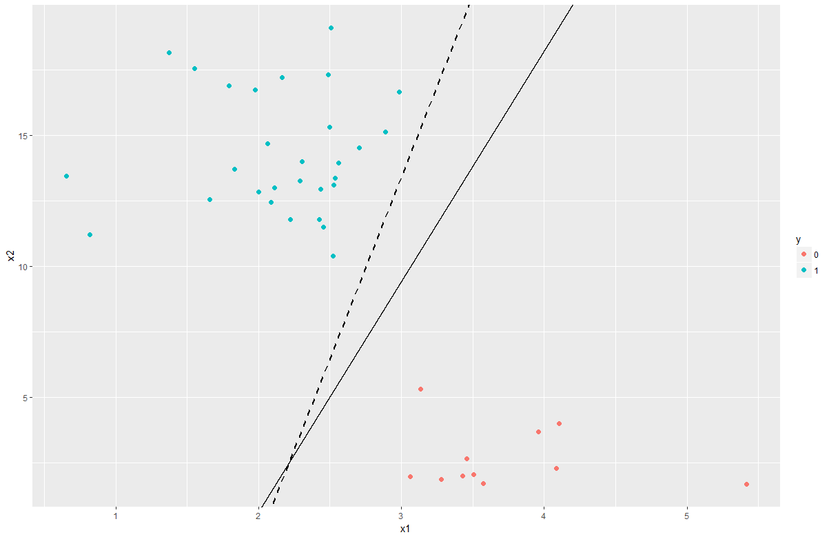
And you can see that logistic regression is a linear classification method: the points on decision boundary is when \(P(y_{i}=1|\mathbf{x}_{i})=1/2\), where leads to \(\mathbf{x}_{i}^\top\mathbf{w}=0\), therefore it’s produce linear decision boundary.