Bagging and Random Forest are one type of ensemble algorithms, they combine the weak learners (decision trees) by averaging or voting their predictions. Bagging is based on bootstrap, resamples data with replacement as new training data for individual trees. Random Forest is based on Bagging and feature subsample at each tree node split.
1. Introduction
Bagging and Random Forests are regarded as implementation of Collective Intelligence. Which means rather than single model, now we get many models in our hand. The names of these two algorithms are intuitive: for “Bagging”, image that we have a “bag” of decision trees and let them work together (actually “bagging” is for “bootstrap aggregation”); for “random forests” we have similar description, we are now facing “forests” rather than single tree.
2. Mathematical Basis
2.1 Bootstrap and Bagging
First let’s introduce bootstrap, it is the base of this two algorithms. Bootstrap is a widely used method in statistics and other fields and it related to “Resampling”. One example is parameter estimation. Consider we have a random sample and we would like to estimate the population mean. We usually use sample mean as the estimation of population mean since this is the “MLE”. But what if we want to know how confidence are we to this estimation? Well we might assume that the sample mean has Normal distribution, using Central Limit Theorem and do some inference; or we can switch to Bayesian statisticians, set up a prior and we observe the data and then simulate the posterior. And we can also use bootstrap. Here is the idea:
- We sample our data with replacement and get a new sample with same sample size, therefore it’s possible that there are duplicates in new sample;
- Repeat this process multiple times, say \(B\). And finally we will have \(B\) samples;
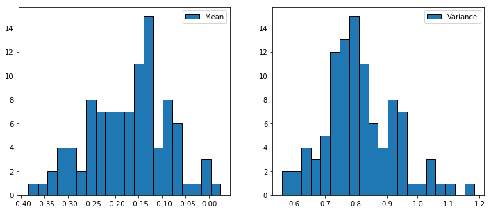
- Get all sample means from these \(B\) samples, now we can form a distribution and do what we want to do (calculate standard deviation).
Here is one simple example:
|
|
where we just get one point… what about using bootstrap?
Ok, now let’s see how bootstrap is incorporated in Bagging.
We can generate \(B\) bootstrap samples and build a decision tree on each of them, then aggregation to get the final result. Yes we can formulate the idea of bagging into one sentence.
The prediction of bagging is given by
\[
\hat{y}_{\text{bag}} = \frac{1}{B}\sum^{B}_{b=1}\hat{y}^{b}
\]
for regression problem, and
\[
\hat{y}_{\text{bag}} = \arg\max_{k}\hat{p}_{k}
\]
for classification problem, where \(\hat{p}_{k}\) is the proportion of \(k\) th category (Majority Vote).
Then we check if there is any problems in this process. Since we use bootstrap, is that possible that some data is not sampled? Yes it is. Consider we have \(n\) data points, the probability that point \(i\) is not selected in one draw is
\[
P(i\text{ not selected in one draw}) = 1 - \frac{1}{n}.
\]
then the probability that this point is not sampled in bootstrap sample is
\[
P(i\text{ not sampled in one bootstrap sample}) = \left(1 - \frac{1}{n}\right)^{n}.
\]
do you see something familiar?
\[
\lim_{n\rightarrow\infty}\left(1-\frac{1}{n}\right)^{n} = \frac{1}{e} \approx 0.367.
\]
This implies that approximately 63% of data is used in Bagging (just approximation!). The rest of data that we are not used is called out-of-bag (OOB) data. It’s important to know how well does bagging perform on the out-of-bag, we need to estimate out-of-bag-error. It can be shown that with B sufficiently large, OOB error is virtually equivalent to leave-one-out cross-validation error\(^{[1]}\).
2.2 Random Forest
Then let’s see Random Forests.
The key word is “Random”, which means at each step of growing tree (find a split), we only use a subset of features rather than all of them, other steps are same as Bagging, this is the only difference between Random Forest and Bagging.
In practice, the sample size for features is denoted as max_features (in sklearn or randomForest (R)), this is one of the hyper-parameters of random forests algorithms. Usually we started with \(m=\sqrt{p}\).
3. Connection between Bagging and Random Forests
If we set the sample size of features equal to the total number of features, random forests is same as bagging.
We can see the difference between bagging and random forests is the number of features. Random forests can de-correlates the decision trees using sampling. Since it is possible that there is an important feature and it will dominant all decision trees if we just include all features, the decision trees are less diversity.
4. Summary
4.1 Pros and Cons
The good things about bagging and random forest:
- Good accuracy because of ensemble mechanism;
- Reduce variance because of bootstrap on samples and features, the variance of random variable mean is scaled by the number of observations;
- Can be trained in parallel;
But:
- Loss of interpretations because of ensemble machanism.
4.2 Feature Importance
Decision tree training is done by recursively splitting, and splitting is done by selecting the combination of feature and value that reduce the most error (impurity). This quantity could be recorded along with each feature across all decision tree, the higher this quantity is the more important the feature it is. This method is by default used in sklearn and other tree ensemble algorithms such as XGBoost and LightGBM.
5. Implementation
The implementations of bagging and random forests are based on decision tree, I invoke DecisionTreeClassifier in sklearn and here is the implementation.
6. References
- Gareth James, Daniela Witten, Trevor Hastie, Robert Tishirani, Introduction to Statistical Learning.
- Random Forest, https://en.wikipedia.org/wiki/Random_forest