A classification method with straightforward geometric intuition.
1. Introduction
Similar with the Logistic Regression we discussed before, SVM is also an algorithm that try to fit a decision boundary to separate the data (as a classifier): define the parameter and loss function, and use optimization algorithm to minimize the loss and learn the parameters, the result would be a decision boundary specified by the parameters.
The extra point is classifying different classes as far as possible, i.e. we need to maximize the distance between the decision boundaries to each class, not just give correct predictions. In other words, a margin is required for the decision boundary. Take binary classification as an example, our ideal decision boundary should locate at the middle of two classes, like the following figure
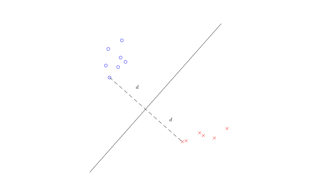
As the figure shows, we will first find a closest pair of points between two classes, and place the decision boundary perpendicular to the connection line between these two points. In order to maximize the distance of decision boundary to each class, we should place the decision boundary at the middle point of the connection line. In this example, the maximum distance is \(d\), and we define it as margin. This classifier is known as Maximum Margin Classifier, it’s a special case of SVM.
Looks nice, but what if the data is not linearly separable? In that case we are not able to conduct the above procedure. Don’t worry, we will back to this point later.
2. Mathematical Basis
2.1 Geometric Interpretation
First we need some geometric backgrounds. Usually we can specify the decision boundary, which is line or hyper plane, using a norm vector \(\mathbf{w}\), and consider a data point \(\mathbf{x}\)
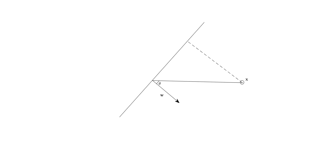
from the figure we can get the following relation (law of cosine):
\[
\cos{\theta} = \frac{\mathbf{w}^{\top}\mathbf{x}}{||\mathbf{w}||_{2}^{2}||\mathbf{x}||_{2}^{2}}
\]
where \(||\mathbf{w}||_{2}^{2}\) means the length of vector \(\mathbf{w}\). So what’s the distance of data point \(\mathbf{x}\) to the decision boundary? We have
\[
d = ||\mathbf{x}||_{2}^{2} \cos{\theta} = \frac{\mathbf{w}^{\top}\mathbf{x}}{||\mathbf{w}||_{2}^{2}}
\]
Also we can observed that whether \(\theta\) is greater than \(\pi/2\) will indicate which side of the decision boundary that \(\mathbf{x}\) located in.
2.2 As a Classifier
This motivate us that the classifier could be
\[
f(\mathbf{x}) = \mathbb{I}\left(\mathbf{w}^{\top}\mathbf{x} > 0\right).
\]
Next we can enter the core part. To fit a decision boundary of SVM (binary), we need to solve the following optimization problem: maximize the margin with the constraints that the distance of every data points to the decision boundary is greater than the margin.
\[
\begin{aligned}
&\max_{\mathbf{w}, b}~\frac{1}{||\mathbf{w}||_{2}^{2}},\\
\text{ s.t. }& y_{i}(\mathbf{w}^{\top}\mathbf{x}_{i} +b)\geq 1, ~i = 1,2,\cdots,n
\end{aligned}
\]
transform to
\[
\begin{aligned}
&\min_{\mathbf{w}, b}~\frac{1}{2}||\mathbf{w}||_{2}^{2},\\
\text{ s.t. }& y_{i}(\mathbf{w}^{\top}\mathbf{x}_{i} +b)\geq 1, ~i = 1,2,\cdots,n
\end{aligned}
\]
where \(y_{i}\) is class label that takes in \(\{-1, +1\}\) (if we use 0 as before, it will get 0 and we will not know which class that this point belongs to). Also we fixed \(\mathbf{w}^{\top}\mathbf{x}=1\), therefore we just need to minimize the denominator. Note: the margin here is geometric margin, there is another margin called functional margin, defined as \(\gamma’ = y(\mathbf{w}^{\top}\mathbf{x}+b)\), geometric margin is defined as \(\gamma = \gamma’ / ||\mathbf{w}||_{2}^{2}\)
And we define the correct classification to be \(y_{i}(\mathbf{w}^{\top}\mathbf{x}_{i} +b)\) to be greater than 1 rather than 0. This is useful in the later discussion, here you just need to know that we generate two parallel lines at both sides of the decision boundary. Therefore we will get the classification result like this,
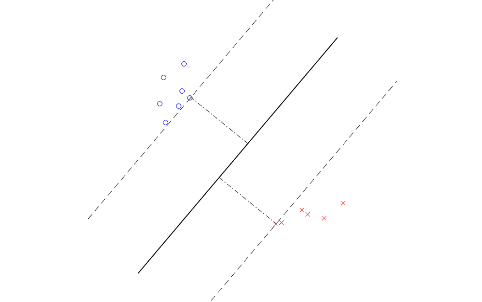
The classifier we got is known as Maximum Margin Classifier. The length of the margin is the distance between the solid line (decision boundary) and the dashed line. The constraints here means the points cannot exceed the margin. And the points on the margin are called support vectors.
2.3 Parameters Estimation by Optimizations with Constraints
Solving this optimization problem is not easy since the constraints are functions. Using Lagrange multipliers we can rewrite optimization problem:
\[
\min_{\mathbf{w}, b} ~\ell = \frac{1}{2}||\mathbf{w}||_{2}^{2} - \sum^{n}_{i=1}\alpha_{i}[y_{i}(\mathbf{w}^{\top}\mathbf{x}_{i} +b) - 1]
\]
take the derivatives respect to \(\mathbf{w}\) and \(c\) we can get
\[
\begin{aligned}
\frac{\partial\ell}{d\mathbf{w}} = \mathbf{w} - \sum^{n}_{i=1}\alpha_{i}y_{i}\mathbf{x}_{i}=0&~\Longrightarrow \mathbf{w}=\sum^{n}_{i=1}\alpha_{i}y_{i}\mathbf{x}_{i} \\
\frac{\partial\ell}{d b} = -\sum^{n}_{i=1}\alpha_{i}y_{i}=0&~\Longrightarrow \sum^{n}_{i=1}\alpha_{i}y_{i}=0
\end{aligned}
\]
Plugging into the previous optimization problem we can again rewrite our optimization problem like this
\[
\begin{aligned}
&\max_{\alpha_{i}}~L = \sum^{n}_{i=1}\alpha_{i} - \frac{1}{2}\sum^{n}_{i=1}\sum^{n}_{j=1}\alpha_{i}\alpha_{j}y_{i}y_{j}\mathbf{x}_{i}^{\top}\mathbf{x}_{j},\\
\text{ s.t. }&~\sum^{n}_{i=1}\alpha_{i}y_{i}=0,~i=1,2,\cdots,n.
\end{aligned}
\]
2.4 Linear or Non-linear Classifier
The solution of this optimization problem exists only the data is linearly separable. If the data is not perfectly linearly separable, we need to modify the constraints and objective functions of the optimization problem.
\[
\begin{aligned}
&\min_{\mathbf{w}, b, \epsilon_{i}}~\frac{1}{2}||\mathbf{w}||_{2}^{2} + \alpha\sum^{n}_{i=1}\epsilon_{i},\\
\text{ s.t. }& y_{i}(\mathbf{w}^{\top}\mathbf{x}_{i} +b)\geq 1-\epsilon_{i}, ~i = 1,2,\cdots,n
\end{aligned}
\]
where \(\alpha\) is our tolerance to the incorrect classification cases; \(\epsilon_{i}\) is called slack variable. \(\epsilon_{i}=0\) when the point is located on the margin. This allows points exist between the decision boundary and margin, even on the other side of the decision boundary.
No we can see if the point is correct classified, we have
\[
y_{i}(\mathbf{w}^{\top}\mathbf{x}_{i}+b)\geq 1\Longrightarrow\epsilon_i=0,
\]
and if the point is not correct classified, we have
\[
y_{i}(\mathbf{w}^{\top}\mathbf{x}_{i}+b) < 1\Longrightarrow\epsilon_{i} = 1-y_{i}(\mathbf{w}^{\top}\mathbf{x}_{i}+b)
\]
therefore we have
\[
\epsilon_{i} = \max\{0, 1 - y_{i}(\mathbf{w}^{\top}\mathbf{x}_{i} + b)\}
\]
We can solve the problem by minimize the overall \(\epsilon_{i}\) and actually we get the loss function of SVM,
\[
L(y_{i}, \hat{y}_{i}) = \max\{0, 1 - y_{i}\hat{y}_{i}\},
\]
this is called hinge loss and it’s a upper bound of 0-1 loss. The following part is easy to go.
3. Implementation
Here is one implementation of linear SVM and demo.
4. Discussions
- Kernel
- Convex Optimization
5. References
- Linear Classification, Standford CS231n, http://cs231n.github.io/linear+blassify/