[Paper reading] Distributed Representations of Words and Phrases and their Compositionality.
1. Introduction
This is the second paper I read about Word2Vec. In the last paper reading note, Mikolov et al presented two models to learn word distributed representations, a.k.a. word embeddings. However, there are several issues - hard to train the model efficiently, cannot get high quality word vectors, etc. In this paper, several tricks are introduced to improve the model training efficiency.
2. Highlights
Some tricks and results:
- by subsampling of frequent words, obtain significant speedup, also learn more regular word representation
- a more efficient computation compared with full softmax: hierarchical softmax; simple alternative to hierarchical softmax: negative sampling
- for inherent limitation of word representation (indifference to word order and their inability to represent idiomatic phrases, present a simple method for finding phrases in text, show that learning good vector representations for millions of phrases is possible)
- simple vector addition can produce meaningful results (e.g. capital of German gives “Berlin”)
2.1 Skip-gram Model
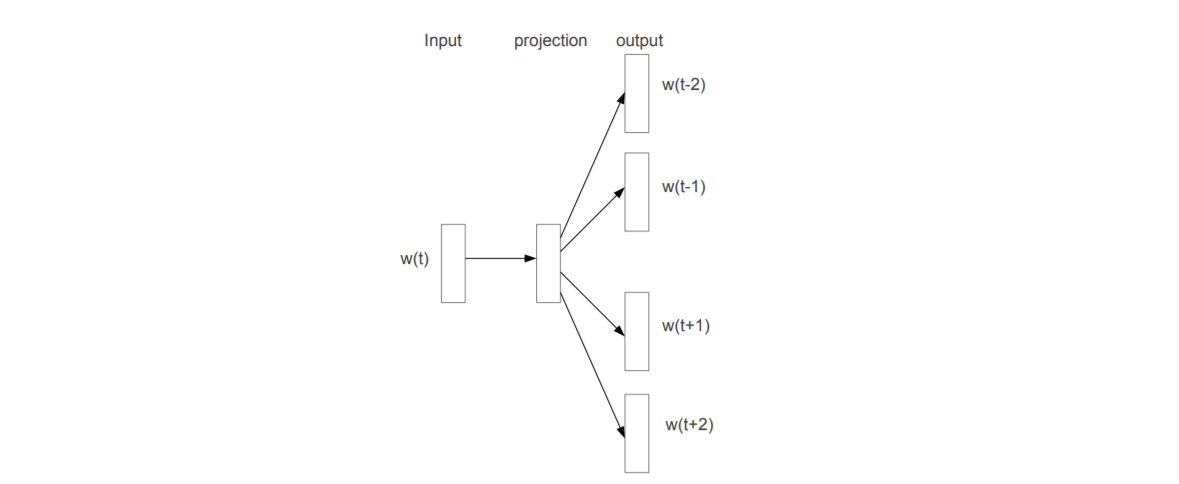
As shown last time, skip-gram model is predict the context based on current word \(w_{t}\). In formal, find word representations that are useful for predicting surrounding words in a sentence or document. Given a sequence of training words \(w_{1}, w_{2},\cdots, w_{T}\), maximize
\[
\frac{1}{T} \sum^{T}_{t=1}\sum_{-c\leq j\leq c, j\neq 0}\log P\left(w_{t+j}|w_{t}\right),
\]
\(c\) is the size of training context, larger \(c\) results in more training examples and thus can lead to higher accuracy.
The probability of context given current word is defined as
\[
P(w_{O}|w_{I}) = \frac{\exp\left(v’^\top_{w_{O}}v_{w_{I}}\right)}{\sum^{W}_{w=1}\exp\left(v’^\top_{w_{w}}v_{w_{I}}\right)}
\]
\(v_{w}\) and \(v’_{w}\) are the “input” and “output” vector representation of \(w\), you can simple think it to be the left side weight and right side weight around the projection layer. \(W\) is the number of words in vocabulary.
2.2 Hierarchical Softmax
This is a computationally efficient approximation for full softmax. In full softmax, the width of the layer is \(W\), and the index of highest probability is the prediction index of word in vocabulary. Use better data structure could improve the computation. Bengio et al previous use binary tree representation. Here they use similar way, use Huffman tree to represent the output layer with \(W\) words as its leaves, for each node, explicitly represents the relative probabilities of its child nodes. So calculate the softmax output of a word is actually along a path from the root to leaf.
Let \(n(w, j)\) be the \(j\)th node on path from root to \(w\), \(L(w)\) be the length of the path (equivalent to the depth of the tree which is \(O(\log W)\)), so \(n(w, 1)\) is root, \(n(w, L(w))\) is \(w\). For any inner node, let \(ch(n)\) be an arbitrary fixed child of \(n\) and let \(\mathbb{[} x\mathbb{]}\) be 1 if \(x\) is true and -1 otherwise. Then hierarchical softmax define
\[
P(w_{O}|w_{I}) = \prod^{L(w)-1}_{j=1}\sigma\left(\mathbb{[}n(w, j+1) = ch\left(n(w, j)\right) \mathbb{]}v’^\top_{n(w,j)} v_{w_{I}}\right)
\]
where \(\sigma(x) = 1 / (1 + e^{-x})\) is the sigmoid function. It can be verified that \(\sum^{W}_{w=1}P(w|w_{I}) = 1\).
The probability definition looks complex, but the intuition is simple. Use the figure from
Xin Rong, word2vec Parameter Learning Explained (this is the paper that strongly recommended if you have difficulities in understanding Word2Vec),
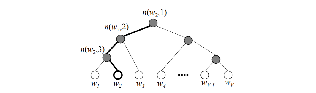
it’s very straightforward to see that the probability of output to be \(w_{2}\) is
\[
P(w_{O}=w_{2}) = P\left(n(w_{2}, 1)\text{ goes left}\right)P\left(n(w_{2}, 2)\text{ goes left}\right)P\left(n(w_{2}, 3)\text{ goes right}\right)
\]
this is equivalent to
\[
P(w_{O}=w_{2}) = \sigma\left(v’^\top_{n(w_{2}, 1)}v_{w_{I}}\right) \sigma\left(v’^\top_{n(w_{2}, 2)}v_{w_{I}}\right) \sigma\left(-v’^\top_{n(w_{2}, 3)}v_{w_{I}}\right)
\]
use property of sigmoid function that \(\sigma(x) + \sigma(-x) = 1\).
2.3 Negative Sampling
An alternative to hierarchical softmax is Noise Contrastive Estimation (NCE). NCE can be shown to approximately maximize log probability of softmax, the skip-gram model is only concerned with learning high quality word vectors, so it’s free to simplify NCE as long as vector representation retain the quality. The task is to distinguish target word \(w_{O}\) from draws from noise distribution \(P_{n}(w)\) use logistic regression, where there are \(k\) negative samples for each positive sample.