[Paper reading] XGBoost: A scalable Tree Boosting System.
XGBoost is a open source software library which provides a gradient boosting algorithm framework. I won’t tell you how powerful it is since I cannot finish it in this small space, but the important factor behind its success is its scalability in all scenarios. It won John Chambers Award and High Energy Physics meets Machine Learning award in 2016. Here is the github repo, documents and published paper.
1. Introduction
Gradient tree boosting, a.k.a. gradient boosting machine (GBM) is a powerful algorithm in many applications. This paper describe XGBoost with innovations:
- a novel tree learning algorithm for handling sparse data
- a theoretically justified weighted quantile sketch procedure enables handling instance weights in approximate tree learning
- an efficient cache-aware block structure for out-of-core tree learning
2. Tree Boosting in a Nutshell
2.1 Regularized Learning Objective
With input data \(\left\{(X_{i}, y_{i}), ~i=1,2,\cdots,n; ~X_{i}\in R^{m}, y_{i}\in R\right\}\), a tree ensemble model with \(K\) additive functions to predict the output
\[
\hat{y}_{i} = \sum^{K}_{k=1}f_{k}\left(X_{i}\right),
\]
where \(f_{k}\) is in the space of regression trees \(\mathcal{F}\), where \(\mathcal{F} = \left\{f(x) = w_{q(x)}\right\}\), \(q: R^{m}\rightarrow T\) and \(w\in R^{T}\). \(q\) denotes structure of the regression tree that maps a input \(x\) to leaf node. \(T\) is the number of leaves. Each tree contains a score on each leaf, \(w_{i}\) is the score of \(i\) th leaf, i.e. for a specific sample, it will go through the regression tree and get to a leaf with a final prediction \(w_{i}\)..
The \(f_{k}\) is from optimizing the objective function:
\[
\mathcal{L} = \sum^{n}_{i=1}l\left(\hat{y}_{i}, y_{i}\right) + \sum_{k}\Omega\left(f_{k}\right),
\]
where \(l\) is a differentiable loss function, and \(\Omega\) plays as regularization term,
\[
\Omega\left(f_{k}\right) = \gamma T + \frac{1}{2}\lambda ||w||^{2}.
\]
2.2 Gradient Tree Boosting
- Setup loss function
Training GBM is sequentially. Let \(\hat{y}_{i}^{(t)}\) be the prediction of input \(X_{i}\) at \(t\) th iteration, a regression tree is trained and add to the output model of \((t-1)\) th iteration, the objective function is:
\[
\mathcal{L}^{(t)} = \sum^{n}_{i=1}l\left(y_{i}, \hat{y}_{i}^{(t-1)} + f_{t}\left(X_{i}\right)\right) + \Omega\left(f_{t}\right) = \sum^{n}_{i=1}l\left(y_{i}, \hat{y}_{i}^{(t)} \right) + \Omega\left(f_{t}\right).
\]
When the loss function \(l\) is squared loss or exponential loss, the calculation is easy, take squared loss as an example:
\[
l\left(y_{i}, \hat{y}_{i}^{(t-1)} + f_{t}\left(X_{i}\right)\right) = \left(y_{i} -\hat{y}_{i}^{(t-1)} -f_{t}\left(X_{i}\right) \right)^{2} = \left(r_{i}^{(t-1)} -f_{t}\left(X_{i}\right) \right)^{2},
\]
where \(r_{i}^{(t-1)}\) is the training residual at iteration \((t-1)\), and you can observe that the goal at iteration \(t\) is to fit a regression tree to the residual from last iteration. Also it is easy to see
\[
-\frac{\partial l\left(y_{i}, \hat{y}_{i}^{(t-1)} \right)}{\partial \hat{y}_{i}^{(t-1)}} = y_{i} - \hat{y}_{i}^{(t)} = r_{i}^{(t-1)},
\]
this means the residual is also the gradient of the loss function which is calculated during training (if use gradient descent based algorithms).
However, sometimes the loss functions are complicated, therefore residual is not equivalent to gradient. GBM can handle other types of loss functions, and the target it use is negative gradient, so every single step - the regression tree is fit on negative gradient, no more “residual” . In some contexts it is also called pseudo-residual, I guess we usually just use “residual” in regression problem, and it could say negative gradient here is the approximation of residual.
In XGBoost framework, they use second-order approximation for objective function:
\[
\begin{aligned}
\mathcal{L}^{(t)} =& \sum^{n}_{i=1} \left[ l\left(y_{i}, \hat{y}_{i}^{(t-1)} + f_{t}(X_{i})\right)\right] + \Omega\left(f_{t}\right) \\
\approx& \sum^{n}_{i=1} \left[ l\left(y_{i}, \hat{y}_{i}^{(t-1)}\right) + g_{i}f_{t}\left(X_{i}\right) + \frac{1}{2}h_{i}f^{2}_{t}\left(X_{i}\right) \right] + \Omega\left(f_{t}\right),\\
\end{aligned}
\]
where
\[
g_{i} = \frac{\partial l\left(y_{i}, \hat{y}_{i}^{(t-1)} \right)}{\partial \hat{y}_{i}^{(t-1)}}, ~h_{i} = \frac{\partial^{2} l\left(y_{i}, \hat{y}_{i}^{(t-1)} \right)}{\partial \left(\hat{y}_{i}^{(t-1)}\right)^{2}}
\]
are the 1st and 2nd order gradient statistics on the loss function. Removing the constant term,
\[
\mathcal{L}^{(t)} \approx \sum^{n}_{i=1} \left[ g_{i}f_{t}\left(X_{i}\right) + \frac{1}{2}h_{i}f^{2}_{t}\left(X_{i}\right) \right] + \Omega\left(f_{t}\right).
\]
Define \(I_{j} = \left\{i | q(x_{i}) = j\right\}\) as samples of leaf \(j\), then the objective function is
\[
\begin{aligned}
\mathcal{L}^{(t)} &\approx \sum^{n}_{i=1} \left[ g_{i}f_{t}\left(X_{i}\right) + \frac{1}{2}h_{i}f^{2}_{t}\left(X_{i}\right) \right] + \gamma T + \frac{1}{2}\lambda\sum^{T}_{j=1}w_{j}^{2} \\
& = \sum^{T}_{j=1}\left[ \left(\sum_{i\in I_{j}} g_{i}\right)w_{j} + \frac{1}{2}\left(\sum_{i\in I_{j}} h_{i} + \lambda\right)w_{j}^{2} \right] + \gamma T.
\end{aligned}
\]
This step shows that train \(f_{t}(X_{i})\) by minimizing loss over all samples is equivalent to heuristically find the best \(f_{t}(X_{i})\) at each step \(t\) - it shows single regression tree learning is part of the sequential learning in XGBoost (it should be true for general gradient boosting algorithms learning).
- Minimizing total loss & Training single regression tree
For a fixed structure regression tree \(q(x)\), the optimal weight of leaf \(j\) is
\[
w_{j} = -\frac{\sum_{i\in I_{j}} g_{i}}{\sum_{i\in I_{j}} h_{i} + \lambda}
\]
with corresponding optimal value
\[
\mathcal{L}^{(t)}(q) = -\frac{1}{2}\sum^{T}_{j=1} \frac{\left(\sum_{i\in I_{j}} g_{i}\right)^{2}}{\sum_{i\in I_{j}} h_{i} + \lambda} + \gamma T.
\]
This equation can be used as a scoring function to measure the quality of a tree structure, like impurity score.
Then the node are splited into left and right branches, suppose \(I_{L}\) and \(I_{R}\) are the samples of left and right child nodes, let \(I = I_{L}\cup I_{R}\), the loss reduction after split is
\[
\mathcal{L}_{\text{split}} = \frac{1}{2}\left[ \frac{\left(\sum_{i\in I_{L}} g_{i}\right)^{2}}{\sum_{i\in I_{L}} h_{i} + \lambda} + \frac{\left(\sum_{i\in I_{R}} g_{i}\right)^{2}}{\sum_{i\in I_{R}} h_{i} + \lambda} - \frac{\left(\sum_{i\in I} g_{i}\right)^{2}}{\sum_{i\in I} h_{i} + \lambda} \right] - \gamma
\]
2.3 Shrinkage and Subsampling
Besides the approximation and regularized objective function, compared with regular GBM, XGBoost also apply two tricks to prevent overfitting:
- Shrinkage: multiply a weight (between 0 and 1) to each new added tree to reduce the influence of individual tree for further trees to improve the model, this weight is usually also interpreted as learning rate. Notice that this weight is added in the loss function rather than model form, the model is still
\[
\hat{y}_{i} = \sum^{K}_{k=1}f_{k}\left(X_{i}\right),
\]
- Subsampling: this is same with Random Forest (bootstrap), with both samples and features get sampled when fitting a new regression tree.
3. Split Finding Algorithm
The most important part in fitting a regression tree is to find a split: which feature to split and what value as split threshold.
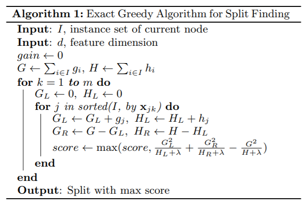
3.1 Basic Extra Greedy Algorithm
The dumpiest way to find the split is brute-force: enumerate over all the possible splits on all features. This is what sklearn, R do. Single machine version of XGBoost also support this algorithm.
3.2 Approximate Algorithm
To make it possible to let the large dataset entirely into memory during split finding, an approximate algorithm is proposed.
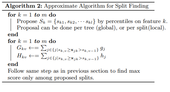
To summarize, the algorithm first proposes candidate splitting points according to percentiles of feature distribution. The algorithm then maps the continuous features into buckets split by the candidate points, aggregate the statistics and find the best solution among proposals based on the aggregated statistics.
3.3 Weighted Quantile Sketch
This part related to the approximation algorithm. I’ll temporary skip this part. TO BE CONTINUED…
3.4 Sparsity-aware Split Finding
There are multiple possible causes for data sparsity:
- presence of missing data
- frequent 0 entries in statistics
- artifacts of feature engineering such as one-hot encoding
XGBoost add a default direction for each tree node. When a feature value is missing, the sample is classified into the default direction. There are two choice for default direction, the optimal is learnt from data: choose the direction to minimize loss. The key improvement is to only visit the non-missing entries. The presented algorithm treats the non-presence as missing value and learns the best direction to handle missing values.
4. System Design
This part is skipped here since I don’t have too much experience in system design :) But this part is very important for XGBoost.
5. Experiments and Conclusions
In the paper, for classification task on single machine, XGBoost is evaluated on Higgs-1M data. Both XGBoost and sklearn give bettern performance than R‘s GBM, while XGBoost runs more than 10x faster than sklearn.
In summary, the paper proposed XGBoost - a scalable tree boosting system. Highlights include:
- a novel sparsity aware algorithm for handling sparse data.
- a theoretically justified weighted quantile sketch for approximate learning.
- experiments show that cache access patterns, data compression and sharding are essential elements for building a scalable end-to-end system for tree boosting.