A practical comparison of XGBoost and LightGBM.
1. Introduction
Last two posts are XGBoost and LightGBM paper readings, they are official descriptions of these two GBM frameworks. However many practical details are not mentioned or described very clearly. Also, there are some different features between them. Therefore this time I’ll give a summary of comparison which will start from their mechanism and practical usage.
2. Common Tricks
2.1 Tree Growing
Both XGBoost and LightGBM support Best-first Tree Growth, a.k.a. Leaf-wise Tree Growth. Many other GBM implementation use Depth-first Tree Growth, a.k.a. Depth-wise Tree Growth. Use the description from LightGBM doc:
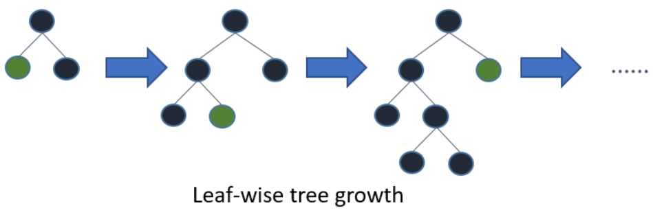
For leaf-wise method, it will choose the leaf with max loss reduce to grow, rather than finish the leaf growth in same level. With number of leaves fixed, leaf-wise method tend to achieve lower loss than depth-wise method. Also leaf-wise method can converge much faster, but it will also be more likely to overfit.
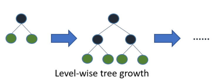
Here is the depth-wise tree growth.
Unlike LightGBM, XGBoost also support depth-wise. The parameter is grow_policy with default to be depthwise; to use leaf-wise, switch to lossguide.
For leaf-wise tree growth, the key parameters are:
- number of leaves:
- XGBoost:
max_leaves(need to setgrow_policy=lossguide, otherwise it is 0) - LightGBM:
num_leaves
- XGBoost:
- max depth:
- XGBoost:
max_depth(can set to 0 whengrow_policy=lossguideandtree_method=hist) - LightGBM:
max_depth(set to -1 means no limit)
- XGBoost:
- min data required in leaf to split:
- XGBoost:
min_child_weight - LightGBM:
min_data_in_leaf
- XGBoost:
2.2 Histogram-based Split Finding
Both XGBoost and LightGBM support histogram-based algorithm for split finding. As mentioned in XGBoost paper, the exact-greedy (brute-force) split find algorithm is time consuming: for current feature to search, need to sort feature values and iterate through. For faster training, histogram-based algorithm is used, which bucket continuous feature into discrete bins. This speeds up training and reduces memory usage.
LightGBM is using histogram-based algorithm. Related parameters are:
max_bin: max number of bins that feature values will be bucketed in.min_data_in_bin: minimal number of data inside one bin.bin_construct_sample_cnt: number of data that sampled to construct histogram bins.
XGBoost has options to choose histogram-based algorithm, it is specified by tree_method with options:
auto: (default) use heuristic to choose the fastest method.exact: exact greedy algorithm.approx: approximate greedy algorithm using quantile sketch and gradient histogram.hist: fast histogram optimized approximate greedy algorithm, with this option enabled,max_bin(default 256) could be tuned
2.3 Missing Values Handling
Both XGBoost and LightGBM could handle missing values in input data.
XGBoost supports missing values by default. As mentioned in the paper, the missing values will be hold at first, then the optimal directions are learning during training to get best performance. On the other hand, XGBoost accepts sparse feature format where only non-zero values are stored, this way the data non-presented are treated as missing.
LightGBM has several parameters for missing values handling:
use_missing: default to betrue.zero_as_missing: default to befalse, which means onlynp.nanis considered as missing.
3. Different Tricks
3.1 Categorical Feature Handling
XGBoost currently only supports numerical inputs, which means if the categorical features are encoded as integers, they are treated as ranked numerical features, this could introduce bias. Therefore one-hot encoding needs to be applied before feed into XGBoost.
LightGBM supports categorical input type, use categorical_feature, notice:
- only supports integer type, e.g. outputs from
sklearn.LabelEncoder. - index starts from 0 and it doesn’t count the label column when passing type is integer.
- all values should be less than
Int32.MaxValue(214783647). - all negative values will be treated as missing value.
In LightGBM, how to find best split for categorical features is briefly described: the optimal solution is to split on categorical feature by partitioning its categories into 2 subsets, if the feature has k categories, there are 2^(k-1)-1 possible partitions, the basic idea is to sort the categories according to training objective at each split; more specifically, it sorts the histogram according to its accumulated values (sum_gradient / sum_hessian) and then finds the best split on the sorted histogram.
And there are also some parameters to handle categorical features regularization.
3.2 Boosters
As mentioned in LightGBM paper, a novel technique called gradient based one-side sampling is used, it could be set by boosting=goss with top_rate (between 0 and 1, the retain ratio of large gradient data) and other_rate (between 0 and 1, the retain ratio of small gradient data) specified.
In XGBoost, there are also multiple options :gbtree, gblinear, dart for boosters (booster), with default to be gbtree.
4. Other Things to Notice
4.1 Feature Importance
Feature importance is a good to validate and explain the results.
LightGBM returns feature importance by calling
the choice of importance_type means different measures of feature importance
"split": the number of times the feature is used to split data across all trees"gain": the total gain of the feature when it is used across all trees
XGBoost returns feature importance by calling
the choice of importance_type includes:
"weight": the number of times the feature is used to split data across all trees"gain": the average gain of the feature when it is used across all trees"cover": the average coverage across all splits the feature is used (relative number of observations related to this feature)"total_gain""total_cover"
5. Summary
There are still other topics worth discussing for XGBoost and LightGBM, e.g. they also both support DART boosting, which could have better performance but the parameter tuning is tricky; e.g. they could not only used on regression and classification tasks, but also learning to rank task. Anyway I’ll update here if there are other interesting comparisons could be done.
Here I also attach two examples of parameters usage for LightGBM and XGBoost.
- LightGBM
|
|
- XGBoost
|
|