Analyzing L1 norm regularization.
The question was raised during this week’s Data Science Read Club of the company. And I found I cannot explain why L1 regularization encourage sparse results to myself, which is no good. Therefore this time I’ll briefly list some explanations from textbooks and websites.
1. Geometric Perspective
I think this interpretation is a “must-read” solution for every people who gets to the materials of comparison between Ridge and Lasso (Least Absolute Shrinkage and Selection Operator), same for me.
From Trevor Hastie, et al The Elements of Statistical Learning page 71:
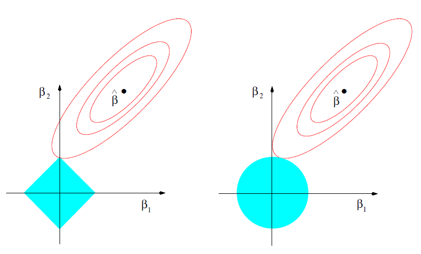
This is a example in 2D case, where the blue area represent the constraint of coefficients: on left: \(|\beta_{1}| + |\beta_{2}| \leq t\), the lasso regression; on right: \(\beta_{1}^{2} + \beta_{2}^{2}\leq t^{2}\), the ridge regression. And the red ellipses are the contours of loss functions. The solution will be the intersection of blue area and red contour. Well, the explanation is:
“The sparsity of L1 regularization is because the solution occurs at corners, then the corresponding coefficients will equal to 0. For high dimensional case there are more corners and there are more opportunities for the coefficients to be 0”
But for me it’s actually not very convincing. Why L2 regularization cannot hit at the corner?
2. Analytical Perspective
2.1 Reduction Norm Perspective
From answer in https://stats.stackexchange.com/questions/45643/why-l1-norm-for-sparse-models, this answer has the highest upvotes.
Consider vector \(x = [1, \epsilon]\) where \(\epsilon > 0\) is a small number. The L1 and L2 norm of \(x\) are given by:
\[
||x||_{1} = 1+\epsilon, ||x||_{2} = 1+\epsilon^{2}.
\]
Then apply a shrinkage on one component:
- Reduce 1 by \(\delta\) and \(\delta < \epsilon\)
The L1 and L2 norm become
\[
||x||_{1} = 1-\delta+\epsilon, ||x||_{2} = 1-2\delta+\delta^{2}+\epsilon^{2}.
\]
- Reduce \(\epsilon\) by \(\delta\) and \(\delta < \epsilon\)
The L1 and L2 norm become
\[
||x||_{1} = 1+\epsilon-\delta, ||x||_{2} = 1+\epsilon^{2}-2\epsilon\delta+\delta^{2}.
\]
Therefore for L1 norm, the shrinkage reduction is same for each coefficient, it move all coefficients towards 0 with same step size, regardless of the quantity being penalized. And for L2 norm, regularizing small term results in a very small reduction in norm, it is highly unlikely that anything will ever be set to zero, since the reducing in L2 norm going from \(\epsilon\) to zero is almost nonexistent when \(\epsilon\) is small.
2.2 Gradient Perspective
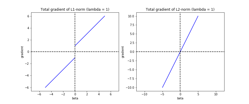
When minimizing loss function, the gradient from regularization term has to be cancelled out to reach the overall zero gradient (indicates minimum loss). For L1 norm, the gradient from regularization part is \(\lambda\) (when \(\beta > 0\)) and \(-\lambda\) (when \(\beta < 0\)). For L2 norm, the gradient from regularization part is \(2\beta\lambda\). So when \(\beta = 0\), the gradient from regularization part is also zero, but the whole gradient is not zero (unlikely?), therefore the optimization algorithm will continue, no sparse solution. But L1 norm has constant gradient, when the constant gradient (\(\pm\lambda\)) is larger than the gradient of fitting term part, it keeps \(\beta = 0\). The chart below can demostrate this:
3. A Simple Example
This example is from the Columbia STAT5241 ML notes.
Suppose \(n=p\), where \(n\) is sample size and \(p\) is feature dimension, input feature matrix is \(X=I\).
For ridge regression, the loss function is
\[
\sum^{p}_{j=1}\left(y_{j} - \beta_{j}\right)^{2} + \lambda\sum^{p}_{j=1}\beta_{j}^{2},
\]
and the solution is
\[
\hat{\beta}_{j} = \frac{y_{j}}{1+\lambda}.
\]
For lasso regression, the loss function is
\[
\sum^{p}_{j=1}\left(y_{j} - \beta_{j}\right)^{2} + \lambda\sum^{p}_{j=1}|\beta_{j}|,
\]
and the solution is depend on the sign of \(\beta\) since absolute value function is not differentiable at origin point.
- If \(\beta_{j} > 0\):
\[
\hat{\beta}_{j} = y_{j} - \frac{\lambda}{2}.
\]
- If \(\beta_{j} < 0\):
\[
\hat{\beta}_{j} = y_{j} + \frac{\lambda}{2}.
\]
In summary we can plot \(y_{j}\) vs \(\beta_{j}\):
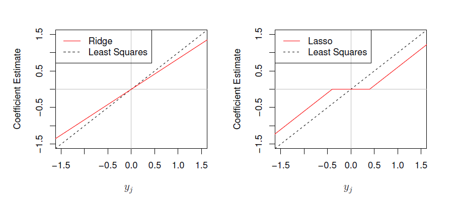
Therefore when \(-\lambda/2 < y_{j} < \lambda/2\) we can see \(\beta_{j} = 0\) which introduces the sparsity.