[Paper reading] Extracting and Composing Robust Features with Denoising Autoencoders.
Recently there is a kaggle competition: Santander Customer Transaction Prediction, the data is totally anonymized. I prefer meaningful features therefore I’m not in this one, but it reminds me of another similar competition: Porto Seguro’s Safe Driver Prediction, where the 1st place solution is pretty cool by using Denoising Autoencoders as a feature extractor to train models. Also I tried apply it in previous work projects, my impression was: it does not need a “bottleneck” structure like basic Autoencoders.
1. Introduction
In previous research, learning deep generative / discriminative models can be difficult, and this could be overcome by an initial unsupervised learning step that maps input features to a latent features. This success appears to be using a layer-by-layer initialization: each layer is first trained to produce a higher level representation of the observed patterns based on the representation it receives as input from the layer below. This technique has been shown empirically to avoid getting stuck in the kind of poor solutions one typically reaches with random initializations.
The explicit criterion to train a good representation includes: retain a certain amount of information about the input. A supplement criterion is the sparsity of the representation. In this paper, a new criterion is proposed: robustness to partial destruction input.
2. Algorithms
2.1 Notations
Let \(X\) and \(Y\) to be two random variables with joint density function \(p(X, Y)\) and marginal density \(p(X)\) and \(p(Y)\). Some notations are defined:
Expectation:
\[
E_{p(X)}[f(X)] = \int p(x)f(x)dx
\]Entropy:
\[
H(X) = H(p) = E_{p(X)}\left[-\log p(X)\right]
\]Conditional entropy:
\[
H(X|Y) = E_{p(X, Y)}[-\log p(X|Y)]
\]Cross entropy:
\[
H(p||q) = E_{p(X)}[-\log q(X)]
\]KL-divergence:
\[
D_{KL}(p||q) = E_{p(X)}\left[\log\frac{p(X)}{q(X)}\right]
\]As you may observe:
\[
H(p||q) = H(p) + D_{KL}(p||q).
\]Mutual information:
\[
I(X; Y) = H(X) - H(X|Y)
\]
2.2 Basic Autoencoder
A basic autoencoder takes an input vector \(\mathbf{x}\in [0, 1]^{d}\) and maps to a hidden representation \(\mathbf{y} = f_{\theta}(\mathbf{x}) = s(\mathbf{Wx} + \mathbf{b})\) with parameter \(\theta\) includes weights \(\mathbf{W}\) and biases \(\mathbf{b}\). Then the hidden representation is mapped back to the reconstructed input \(\mathbf{z}\in [0, 1]^{d}\), which is \(\mathbf{z} = g_{\theta’}(\mathbf{y})=s(\mathbf{W’y} + \mathbf{b’})\) with parameter \(\theta’\) includes weights \(\mathbf{W’}\) and biases \(\mathbf{b’}\). The weight \(\mathbf{W’}\) may optionally be constrainted by \(\mathbf{W’} = \mathbf{W}^\top\) in which case the autoencoder is said to have tied weights.
The parameters are learned by minimizing reconstruction loss:
\[
\theta^{*}, \theta’^{*} = \arg\min_{\theta, \theta’} \frac{1}{n}\sum^{n}_{i=1}L\left(\mathbf{x}_{i}, \mathbf{z}_{i}\right) = \arg\min_{\theta, \theta’} \frac{1}{n}\sum^{n}_{i=1}L\left(\mathbf{x}_{i}, g_{\theta’}\left(f_{\theta}(\mathbf{x}_{i})\right)\right).
\]
Usually the loss function could be squared loss: \(L(\mathbf{x}, \mathbf{z}) = (\mathbf{x} - \mathbf{z})^{2}\). An alternative loss, suggested by the interpretation of \(\mathbf{x}\) and \(\mathbf{z}\) as either bit vectors or vectors of bit probabilities is the cross-entropy:
\[
L(\mathbf{x}, \mathbf{z}) = -\sum^{d}_{k=1}\left(\mathbf{x}_{k}\log \mathbf{z}_{k} + (1 - \mathbf{x}_{k})\log\left(1 - \mathbf{z}_{k}\right)\right).
\]
Here if \(x\) is a binary vector, then \(L(\mathbf{x}, \mathbf{z})\) is a negative log-likelihood of \(\mathbf{x}\) given the Bernoulli distribution parameter \(\mathbf{z}\), then the learning objective is:
\[
\theta^{*}, \theta’^{*} = \arg\min_{\theta, \theta’} E_{q^{0}(X)}[L(X, g_{\theta’}(f_{\theta}(X)))],
\]
where \(q^{0}(X)\) denotes the empirical distribution associatede to \(n\) training inputs.
2.3 Denoising Autoencoder
Now train the autoencoder to reconstruct a clean “repaired” input from a corrupted, partially destroyed one. This is done by first corrupting the initial input \(\mathbf{x}\) to get a partially destroyed version \(\mathbf{\tilde{x}}\) by means of a stochastic mapping \(\mathbf{\tilde{x}}\sim q_{D}(\tilde{\mathbf{x}}|\mathbf{x})\), note that this mapping is only used in training. The corrupted input \(\mathbf{\tilde{x}}\) is then mapped as with the basic autoencoder. And the loss is calculated on raw input rather than corrupted input.
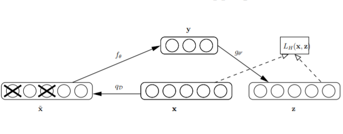
From point of view of the learning steps (gradient descent like algorithms), it’s also random corrputed. In this way, the autoencoder cannot learning the identity function, unlike basic autoencoder, the constraint that \(d’ < d\) can be removed, the latent feature space is not necessary to be “dimension reduced”.
3. Relationship to Other Approaches
- Image Denoising Problem
The problem of image denoising has been extensively studied in the image processing community. The denoising autoencoder’s objective however is fundamentally different from that. The authors investigated explicit robustness to corrupting noise as a novel criterion guiding the learning of suitable intermediate representations to initialize a deep network. Thus the corruption and denoising is applied not only on the input, but also recursively to hidden layers.
- Training Data Augmenting
In contrast to this technique, denoising autoencoder does not use any prior knowledge of image topology, nor does it produce extra labeled examples for supervised training. Denoising autoencoder uses corrupted patterns in a generic unsupervised initialization step, while the supervised training phase uses the unmodified original data.
- Regularization
Training with “noise” and regularization are equivalent for small additive noise. By contrast, corruption in denoising autoencoder is large, non-additive and destruction of information. Also, regularizations in basic autoencoder don’t yield quantitative jump in performance.
Including Manifold Learning Perspective, Top-down & Generative Model Perspective, Information Theoretic Perspective and Stochastic Operator Perspective. I’ll skip this part first.
5. Conclustions
The experiments on image data (convolution neural networks) shows that: without denoising procedure, many filters appear to have learnt no interesting feature. They look like the filters obtained after the random initialization. By increasing the level of destructive corruption, an increasing number of filter resemble sensible feature detectors, they appear sensitive to larger structure spread out across more input dimensions.
In summary, explicit denoising criterion helps to capture interesting structure in the input distribution. This in turn leads to intermediate representations much better suited for subsequent learning tasks such as supervised classification.