Reading notes of “The Beauty of Mathematics in Computer Science” by Dr. Jun Wu. The book is mainly about mathematical applications in real world, including NLP, information theory, information retrieval.
I was a freshman (2012) when I first read this book, to be honest at that time this book didn’t impress me a lot - since I had no basis in this area. Now in 2020, as I’ve been working as a Data Scientist for two years, I read this book again, I’m really impressed and regret I didn’t deep dive into this area when I first read it.
This time I spend three days on reading it, here are some notes I highlighted.
1. Natural Language Processing - From Rule Based to Statistical Based
In 1960s, syntactic and semantic analysis were regarded as two basic dimensions in NLP. In syntactic analysis, as the grammar rules, part of speech, morphologic and etc can be abstracted into algorithms, rule based parsers were built to generate the parse / syntax tree for simple sentences. However it will generate exponential possible solutions for complex sentences in real world, it cannot scale up. Also, natural language cannot be described by context free grammar.
Statistical based parsers were developed started in 1970s. With the power of statistics, more successful NLP applications are developed:
- speech recognition
- machine translation
- syntactic analysis
- …
2. Hidden Markov Model
A communication system with six basic elements in communication process (sender, ideas, encoding, communication channel, receiver, decoding):
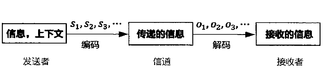
The basic problem is how to inference the source information based on observations:
\[
s_{1}, s_{2}, s_{3}, \cdots = \arg\max_{s_{1}, s_{2}, s_{3}, \cdots} P(s_{1}, s_{2}, s_{3}, \cdots|o_{1}, o_{2}, o_{3}, \cdots).
\]
Using bayes formula:
\[
P(s_{1}, s_{2}, s_{3}, \cdots|o_{1}, o_{2}, o_{3}, \cdots) = \frac{P(o_{1},o_{2},o_{3},\cdots|s_{1}, s_{2}, s_{3},\cdots)P(s_{1},s_{2},s_{3},\cdots)}{P(o_{1},o_{2},o_{3},\cdots)}.
\]
Hidden Markov Model can be used then. Using Markov property:
\[
\begin{aligned}
P(o_{1}, o_{2}, o_{3},\cdots|s_{1}, s_{2}, s_{3},\cdots) &= \prod_{t}P(o_{t}|s_{t}) \\
P(s_{1}, s_{2}, s_{3},\cdots)&=\prod_{t}P(s_{t}|s_{t-1}).
\end{aligned}
\]
In NLP, \(P(s_{1}, s_{2}, s_{3},\cdots)\) is the language model. \(P(o_{1}, o_{2}, o_{3},\cdots|s_{1}, s_{2}, s_{3},\cdots)\) has different names in different areas, it is Acoustic Model in speech recognition; it is Translation Model in machine translation; it is Correction Model in spell correction.
Three basic use cases of Hidden Markov Model:
- given the model, calculate the probability of specific outputs (forward-backward algorithm)
- given the model and observed outputs, find the most likely inputs (Viterbi algorithm)
- estimate the model given sufficient observed data (Hidden Markov Model training)
3. Information Content and TFIDF
The measure of information is called entropy:
\[
H(X) = -\sum_{x}P(x)\log P(x).
\]
In average, the entropy of chinese character is 8 - 9 bits (using 8 - 9 binary number). Consider the context dependent, every chinese character has around 5 bits, there a chinese book with 500 throusands characters has 2.5 million bits.
In web search, the weight of the keyword \(w\) in the query should reflect the informativeness. A simple approach is using the entropy,
\[
I(w) = -P(w)\log P(w) = -\frac{TF(w)}{N}\log\frac{TF(w)}{N} = \frac{TF(w)}{N}\log\frac{N}{TF(w)},
\]
where \(N\) is the size of the vocabulary, it can be ignored since it is a constant. Assume (1) the size of each document \(M\) are same,
\[
M = \frac{N}{D} = \frac{1}{D}\sum_{w}TF(w).
\]
(2) the contribution of keyword in the document is not relevant to the frequency, therefore a word can appear \(c(w) = TF(w) / D(w)\) times (\(c(w) < M\)) or zero times, then
\[
TF(w)\log\frac{N}{TF(w)} = TF(w)\log\frac{MD}{c(w)D(w)} = TF(w)\log\left(\frac{D}{D(w)}\frac{M}{c(w)}\right).
\]
And TFIDF is:
\[
TFIDF(w) = TF(w)\log\frac{D}{D(w)} = I(w) - TF(w)\log\frac{M}{c(w)}.
\]
Therefore the more informative \(w\) is, the larger TFIDF value is; the larger \(c(w)\) is (query keywords match word in documents), the larger TFIDF is. These two conclusions are consistent with the information theory.
4. Text Categorization and SVD
Two common text categorization (clustering) tasks: categorize documents by topics and categorize words by meanings. These two tasks can be done by calculating the cosine similarity of document / word vectors from word-document matrix \(X\).
When the matrix is very large, SVD can be applied:
\[
X = U\Sigma V^\top,
\]
with interpretations:
- matrix \(U\) is the result of words categrization, each row represents a word, each column represents a class with similar word meanings (semantic)
- matrix \(V^{\top}\) is the result of document categorization, each row represents a document, each column represent a topic
I’ve summarized the basic usage of SVD in python here.
5. Maximum Entropy Model
Maximum Entropy principal: when make predictions on probability distributions for random events, no subject assumptions should be made - in this situation, the most uniform distribution has the lowest risk and highest entropy.
The maximum entropy model for next word prediction:
\[
P(w_{3}|w_{1}, w_{2}, s) = \frac{1}{Z(w_{1}, w_{2}, s)}e^{\lambda_{1}(w_{1}, w_{2}, w_{3})+\lambda_{2}(s, w_{3})},
\]
where \(Z\) is the normalization term.