Attention Mechanism: a new network structure - no convolution, no recurrent unit.
1. Attention in Machine Translation
Paper: Neural Machine Translation By Jointly Learning to Align and Translate
This paper proposed using attention mechanism in Seq2Seq model in machine translation, it allows automatically search for parts of a source sentence that are relevant to predicting a target word, without having to form these parts as a hard segment explicitly. It’s the first time I know attention mechanism.
1.1 Seq2Seq - Encoder Decoder Model
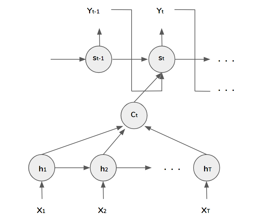
In Encoder-Decoder framework, an encoder reads the input sequence \([x_{1}, x_{2}, \cdots, x_{T}]\), into a context vector \(c\). The most common approach is to use an RNN such that
\[
h_{t} = f(x_{t}, h_{t-1}), c = q(\{h_{1},h_{2},\cdots, h_{T}\}),
\]
where \(h_{t}\in R^{n}\) is a hidden state at time \(t\).
The decoder generates the prediction at time \(t\) given the context vector \(c\) and all the previous predictions \([y_{1}, y_{2}, \cdots, y_{t-1}]\):
\[
p(y_{t}|y_{1}, y_{2},\cdots,y_{t-1}, c) = g(y_{t-1}, s_{t}, c),
\]
where \(g\) is a nonlinear function, \(s_{t}\) is the hidden state of RNN.

Here the context vector serves as initial input for decoder and input for output \(y\) in every step.
1.2 Attention Mechanism
In the new model architecture, the prediction is generated as
\[
p(y_{t}|y_{1}, y_{2},\cdots,y_{t-1}, c) = g(y_{t-1}, s_{t}, c_{t}),
\]
where the hidden state at time \(t\) is calculated by
\[
s_{t} = f(s_{t-1}, y_{t-1}, c_{t}),
\]
the context vector \(c_{t}\) is unique for each step \(t\).

The context vector \(c_{t}\) depends on a sequence of annotations \(\left(h_{1}, h_{2}, \cdots, h_{T_{x}}\right)\) to which an encoder maps the input sentence. Each annotation \(h_{t}\) contains information about the whole input sequence with a strong focus on the parts surrounding the \(t-\)th word of the input sequence.
The context vector \(c_{t}\) is calculated as a weighted sum of the annotations:
\[
c_{t} = \sum^{T_{x}}_{j=1}\alpha_{tj}h_{j},
\]
the weight \(\alpha_{tj}\) of each annotation is calculated by softmax
\[
\alpha_{tj} = \frac{\exp(e_{tj})}{\sum^{T_{x}}_{k=1}\exp(e_{tk})},
\]
where \[
e_{tj} = score(s_{t-1}, h_{j}) = v_{a}^{\top}\tanh\left(W_{a}[s_{t}; h_{j}]\right)
\]
is an alignment model which scores how well the inputs around position \(j\) and the output at position \(t\) match. The score is based the on RNN hiddent state and annotation of the input sentence. The alignment model is parameterized as a feedfoward neural network which is jointly trained with the seq2seq model.
To understand this approach of taking a weighted sum of all the annotation as calculating an expected annotation, the weight \(\alpha_{tj}\) is a probability that the target word \(y_{t}\) is aligned to the source word \(x_{j}\). Intuitively, the decoder decides parts of the source sentence to pay attention to, it lets the model focus only on information relevant to the generation of the next target word.
2. Other Forms of Attention Mechanisms
Paper:
- Neural Machine Translation By Jointly Learning to Align and Translate
- Show, Attend and Tell: Neural Image Caption Generation With Visual Attention
- Effective Approaches to Attention-based Neural Machine Translation
2.1 Deterministic “Soft” Attention and Stochastic “Hard” Attention
In short, soft attention is parameterized, end-to-end differentiable, therefore it can be trained (all components are weighted); hard attention is not (only one component can be selected / attended each time). The attention mechanism in section 1.2 is soft attention.
2.2 Global Attention and Local Attention
In short, global attention indicates all the hidden states are used to calculate the context vector; local attention first predicts the aligned position for current target word to get the context vector. The attention mechanism in section 1.2 is global attention.
2.3 Self-Attention
Unlike traditional attention which is based on the hidden states from source and target, self-attention is calculated within source or target, it captures the relationship of words in the source or target themselves (e.g. current word and previous words in the same sentence), it can be used to compute a representation of the sequence.
3. Attention Is All You Need - Transformer
Paper: Attention Is All You Need
Transformer is a new network structure (for machine translation in original paper) solely based on attention mechanisms, dispensing recurrence and convolutions entirely. Experiments show the model to be superior in quality while being more parallelizable and requiring significantly less time to train.
3.1 Model Architecture
3.1.1 Encoder and Decoder Stacks
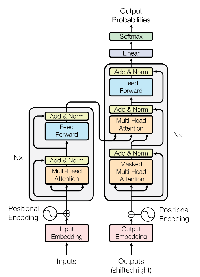
The transformer follows the architecture using stacked self-attention and point-wise, fully connected layers for both the encoder and decoder.

Both encoder and decoder are composed of 6 identical layers. Encoder (left side in the figure) has two sub-layers: multi-head attention (every multi-head attention unit is composed of scaled dot-product attention units) and a position-wise fully connected feedforward network, a residual connection is used around each of the two sub-layers, followed by layer normalization, dimension of the model output is 512. Decoder has the one more sub-layer, which performs multi-head attention over the output of the encoder, the masking ensures that the predictions for position \(i\) can depend only on the known outputs at positions less than \(i\).
3.1.2 Attention
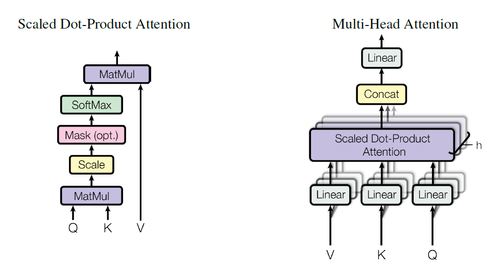
An attention function can be described as mapping a query and a set of key-value pairs to an output. The attention here is called “scaled dot-product attention”, the input consists of queries and keys of dimension \(d_{k}\), and values of dimension \(d_{v}\).

The dot products of the query is calculated across all keys, divide each by \(\sqrt{d_{k}}\) and apply a softmax function to obtain the weights on values:
\[
\text{Attention}(Q, K, V) = \text{softmax}\left(\frac{QK^{\top}}{\sqrt{d_{k}}}\right)V.
\]
The scaling factor \(\sqrt{d_{k}}\) can counteract the effect when \(d_{k}\) is large and the doct products grow large in magnitude (where softmax function is in regions where it has extremely small gradients).
Two commly used attention functions are additive attention and dot-product attention. Additive attention computes the compatibility function using feedforward network with a single hidden layer, while dot-product attention is much faster and more space-efficient in practice, since it can be implemented using highly optimized matrix multiplication code.
Multi-head attention allows the model to jointly attend to information from different representation subspaces at different positions:
\[
\text{MultiHead}(Q, K, V) = \text{Concat}(\text{head}_{1}, \text{head}_{2}, \cdots, \text{head}_{h})W^{O},
\]
where
\[
\text{head}_{i} = \text{Attention}\left(QW_{i}^{Q}, KW_{i}^{K}, VW_{i}^{V}\right),
\]
and \(W_{i}^{Q}\in R^{d_{\text{model}}\times d_{k}}\), \(W_{i}^{K}\in R^{d_{\text{model}}\times d_{k}}\), \(W_{i}^{V}\in R^{d_{\text{model}}\times d_{v}}\) and \(W^{O}\in R^{hd_{v}\times d_{\text{model}}}\).
3.1.3 Positional Encoding
Positional encoding is used to make use of the order of the sequence:
\[
\begin{aligned}
PE_{(pos, 2i)} &= \sin\left(\left(\frac{pos}{10000}\right)^{2i / d_{\text{model}}}\right), \\
PE_{(pos, 2i+1)} &= \cos\left(\left(\frac{pos}{10000}\right)^{2i / d_{\text{model}}}\right)
\end{aligned}
\]
where \(pos\) is the position and \(i\) is the dimension.
3.2 Summary
Applications of attention in the model:
- in encoder-decoder layers, the queries come from the previous decoder layer, the memory keys and values come from the output of encoder. This allows every position in the decoder to attend over all positions in the input sequence
The reason of using self-attention:
- low computational complexity, computation can be parallelized
- easier to learn long-range dependencies (shorter paths between positions in the input and output sequences make it easier to learn long-range dependencies)
- self-attention could yield more interpretable models